THE MATH BEHIND ΕΠΙΔΗΜΙΕΣ

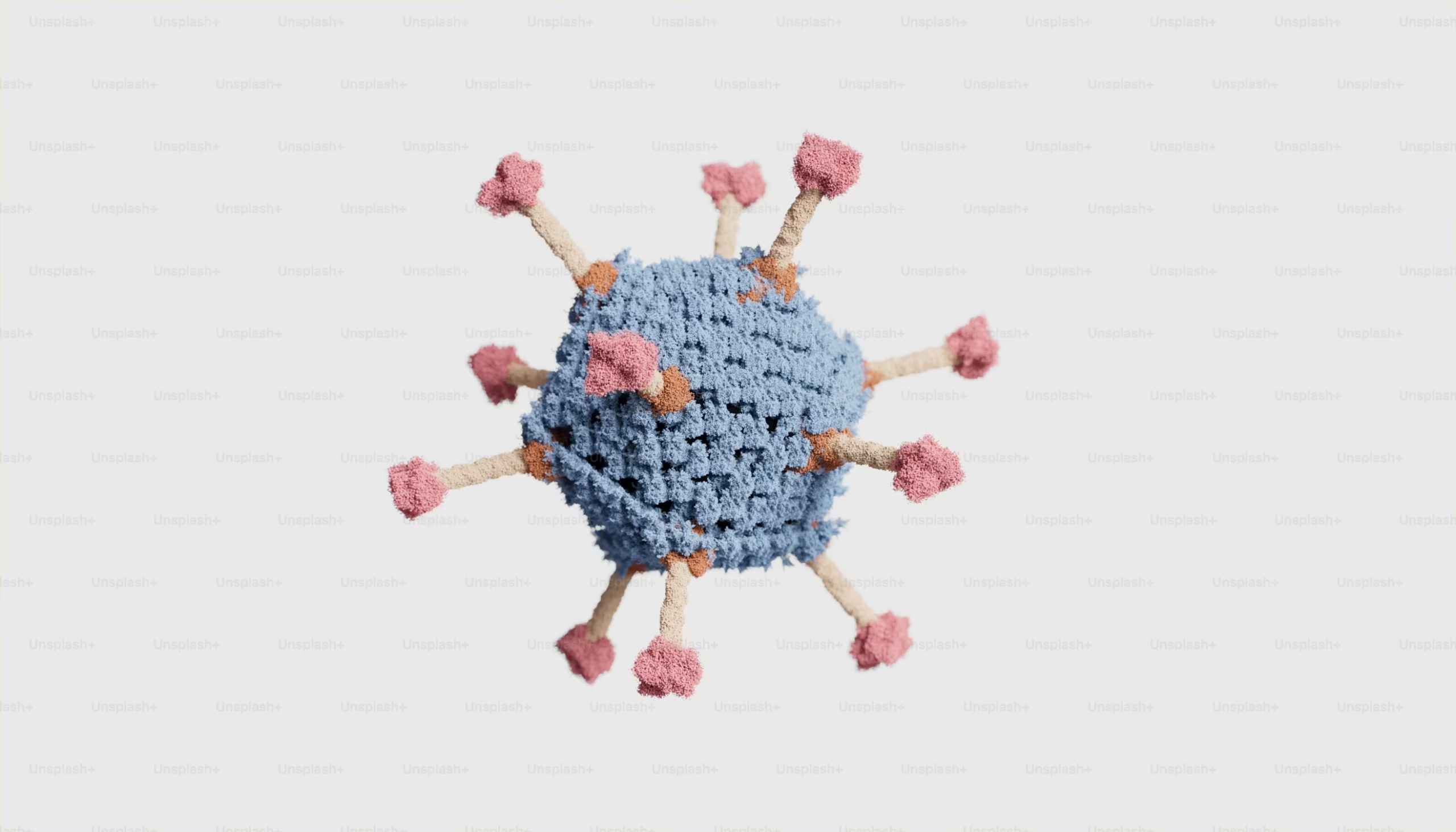
Epidemic modelling involves analyzing the spread of infectious diseases, mathematically.

WHY TRY ANALYZING THE NUMBER OF INFECTIONS?

Epidemic modelling is an essential tool for planning future responses to disease outbreaks. By analyzing past and present data, researchers develop mathematical models that predict how many people are likely to become infected. These predictions help governments and health officials decide whether quarantine measures are needed and estimate how quickly action must be taken.

WHAT DATA DO YOU NEED TO CARRY OUT THIS ANALYSIS?

To start with, you need to find out the total number of people who are healthy, but stand at the risk of contracting the disease (say ‘S(t)’). You also need some additional information:-

Number of infected people (say ‘I(t)’)
Number of immune people (usually the ones who were infected but have now recovered; say ‘R(t)’)

*Note that in the case of some diseases, people who have been infected previously may not stand a better chance of contracting the disease again than a person who has not been infected earlier, but the idea is useful nonetheless.

A RUDIMENTARY MODEL: THE SIR MODEL

Assume that no one is dying due to any cause, i.e., the disease at hand is non-lethal.
Let the total size of the population be N, all of whom are at risk. Then N remains constant by the premise above.

Then, N=S(t)+I(t)+R(t)
Let’s say that 2 people meeting, one infected, the other not, lends a ‘p’ chance of infection to the healthy person, and assume that each person has ‘c’ contacts (contacts include people the infected person meets in 1 day)
Assume that all infected people meet someone according to the rules specified above.
Note that at any time, the fraction of people who are at risk is S(t)/N
Therefore, after 1 day, the number of new infections will be I(t+1)=I(t)[pc][S(t)/N]
Let the mean recovery time be D days (=> there is a 1/D chance of someone recovering each day), then the number of infected people will change per day as

I(t+1)=I(t)+I(t)(pc)(\frac{S(t)}{N})-I(t)(\frac{1}{D})= I(t)[1+(pc)(\frac{S(t)}{N})-\frac{1}{D}]

Now modify the timestep to incorporate any change in time, not just one day
So,

I(t+\Delta t)=I(t)+\left\{I(t)(pc)(\frac{S(t)}{N})-\frac{I(t)}{D}\right\}\Delta t

Note that transforming this equation into a differential equation then yields (assuming S(t) remains relatively constant, equal to S(0))

\frac{dI}{dt}=I(t)\left(\frac{pcS(0)}{N}-\frac{1}{D}\right)

Note that if pcDS(0)>N, the number of infected people grows exponentially, and if pcDS(0)<N, the number of infected people decays exponentially, while pcDS(0)=N implies that the number of infected people remains constant.

What does pcDS(0)=N mean, in the context of the disease? It implies a change in the epidemic’s behaviour: a new strain (pattern).

However how would we expect the number of susceptible people to change? It should change as

\frac{dS(t)}{dt}=-S(t)\left(\frac{pc}{N}I(t)\right)

Why? the term in the brackets represents the proportion of susceptible people which get infected, since this number changes on the basis of the number of infected people at any given time.

Let us examine the above equations in the light of a more general assumption (S(t) changes)

The equations now become

\frac{dI}{dt}=I(t)\left(\frac{pcS(t)}{N}-\frac{1}{D}\right)

and

\frac{dS(t)}{dt}=-S(t)\left(\frac{pc}{N}I(t)\right)

This system of coupled differential equations does not have an elementary solution, because dividing both equations cannot recover the time variable in terms of either S(t) or I(t).

However dividing both equations yields the following relationship, (when coupled with the initial conditions I(0)=1, S(0)=N-1)

I(t)+S(t)-\frac{N}{pcD}\ln\left(S(t)\right) = N-\frac{N}{pcD}\ln\left(N-1\right)

From here it is easy to see that plugging this relation back into the original equations will not yield an elementary antiderivative to compute I(t) or S(t)

However, we also need to recognize the fact that our disease is non-lethal, and therefore the number of susceptible people also reduces by the amount of recovered people i.e., the factor pc/N changes as pc/(N-R(t))=pc/(I(t)+S(t)) since N-S(t)-I(t)=R(t)

This yields the following implicit solution (obviously no time dependent form because of the complexity)

I+S=N\left(\frac{S}{N-1}\right)^{\frac{1}{pcD}}

DISEASE ENDEMICITY AND THE SIS SYSTEM

The SIS system does not impart immunity, and thus non-infected people are simply susceptibles.

The endemic state of a disease is characterized by a steady state solution to the following system of equations

S(t) + I(t) = N

Also, consider the assumption of a vaccine being developed, i.e., introduce a new class V(t), the number of vaccinated individuals.

Let the vaccination rate be ‘ $\nu$ ‘, i.e., people are directly transferred from S(t) to V(t) upon vaccination. Also include fertility as well as mortality at a rate of ‘ $\mu$ ‘

\begin{cases} \displaystyle \frac{dS}{dt} = -\lambda(S(t)) – \nu S(t) + \gamma I(t)+\mu N,\\[8pt] \displaystyle \frac{dI}{dt} = \lambda(S(t)) – (\gamma+\nu) I(t),\\[8pt] \displaystyle \frac{dV}{dt} = \nu (S(t)+I(t))-\mu N, \end{cases} \qquad \begin{aligned} S(0) &= S_0,\\ I(0) &= I_0,\\ V(0) &= V_0. \end{aligned}

Population conservation:

S_0+I_0+V_0=N

Final endemic solution:
At equilibrium,

\frac{dS}{dt} = \frac{dI}{dt} = \frac{dV}{dt} = 0

\boxed{ \left(S^{*},I^{*},V^{*}\right) = \left( \frac{\mu}{\nu} \left( 1-\frac{\lambda}{\gamma+\lambda+\nu} \right)N, \; \frac{\mu}{\nu} \left( \frac{\lambda}{\gamma+\lambda+\nu} \right)N, \; N-\frac{\mu N}{\nu} \right) }

Final recovery solution is the ones where everyone recovers.

admin